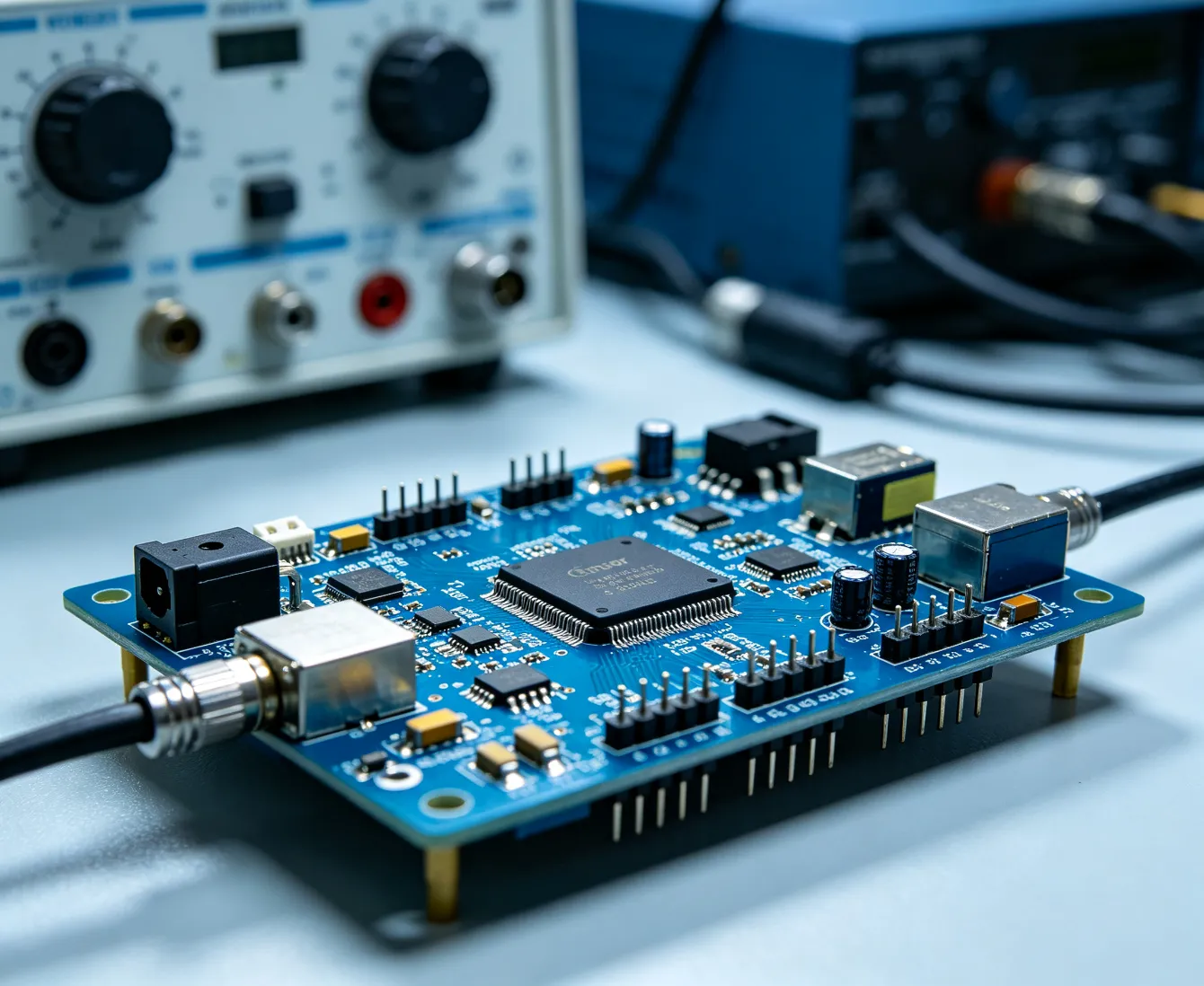
A sensor converts that physical phenomenon into an electrical signal.
But the sensor itself does not determine the quality of the final measurement.
Between the physical world and the final digital value are many engineering stages:
365PCB Sensor & Signal Conditioning Design approaches this complete chain as one measurement system.
A Sensor Produces a Signal.
Engineering Turns That Signal Into a Measurement You Can Trust.
Start With the Physical Quantity
The first engineering question should not be:
Which sensor should we buy?
It should be:
What exactly must the product know?
For example:
“Measure temperature” is not yet a complete requirement.
Engineering needs to understand:
Measurement range
Required accuracy
Resolution
Repeatability
Response time
Sampling rate
operating temperature
environmental exposure
sensor location
calibration requirements
lifetime
cost
production volume
Similarly:
“Measure vibration”
could mean:
or:
Measure a calibrated acceleration spectrum from 1 Hz to 20 kHz.
Those are completely different engineering problems.
Define the Measurement Before Selecting the Sensor.
Sensor Requirements Engineering
A professional sensor-development program can define:
Minimum and maximum physical quantity.
Maximum allowable deviation from the true value.
Smallest meaningful change the system must detect.
How consistently the same input produces the same result.
How quickly the measured phenomenon can change.
How rapidly the product must respond.
How performance changes with:
Temperature + Time + Aging.
Humidity, vibration, contaminants, mechanical loading and other operating conditions.
How long the sensor system needs to remain functional and supportable.
Measurement Requirements Become Sensor Architecture.
Sensor Technology Selection
Different physical phenomena can often be measured using several different sensor technologies.
For temperature:
RTD
Thermocouple
Thermistor
Semiconductor Sensor
For current:
Shunt
Hall Effect
Fluxgate
Current Transformer
For position:
Encoder
Hall
Magnetic
Inductive
Optical
Potentiometric
LVDT
For pressure:
Piezoresistive
Capacitive
MEMS
The correct technology depends on:
Accuracy + Range + Bandwidth + Environment + Cost + Size + Power + Reliability.
The Best Sensor Technology Is Application-Specific.
Sensor Signal-Chain Architecture
A general sensor signal chain may look like:
Analog Devices similarly describes high-performance signal conditioning as critical to systems measuring physical quantities such as temperature, light, chemical phenomena, weight and position, with the signal chain—not merely the sensing element—determining measurement confidence.
The Sensor Is Only the First Electrical Stage.
Sensor Excitation
They need controlled electrical excitation.
Examples include:
Voltage or current excitation.
Precision current excitation.
Controlled bias network.
Voltage bias or zero-bias operation depending on requirements.
AC or switched excitation.
AC excitation.
The excitation source may directly affect accuracy.
If the Sensor Depends on Excitation, the Excitation Is Part of the Measurement.
Ratiometric Sensor Architecture
One powerful technique is:
Ratiometric Measurement.
Suppose a bridge sensor output is proportional to excitation voltage.
If the ADC reference uses the same excitation source, changes in that source can partly cancel mathematically.
Conceptually:
and:
Therefore:
Better Architecture Can Remove an Error Before Calibration Is Needed.
This is particularly powerful for resistive bridge and RTD systems.
Sensor Analog Front End
The AFE sits between the sensor and data converter.
It may include:
Modern sensor AFEs increasingly integrate several of these functions into one device. Current precision sensor-interface ICs can combine programmable gain, ADC, calibration memory, digital processing and multiple analog/digital output options, illustrating how much of traditional sensor conditioning is now becoming integrated and programmable.
Sensor Interface Design Is Becoming Programmable Measurement Architecture.
Gain Architecture
Very small sensor outputs often require amplification.
But amplification should be engineered carefully.
If a sensor produces:
10 mV full scale
and the ADC supports:
2.5 V full scale
a gain of approximately:
250
might appear attractive.
But the engineer must also consider:
sensor offset
overload
common-mode range
amplifier output swing
tolerance
drift
Use the ADC Range Efficiently Without Amplifying the Error Into Saturation.
Programmable Gain
Products with wide dynamic range may use:
PGA — Programmable Gain Amplifier.
Example gain settings:
1×
2×
4×
8×
16×
32×
This can support different:
sensor ranges
product variants
operating modes
But switching gain introduces calibration and settling considerations.
Programmable Gain Creates Flexibility — and Additional States That Must Be Verified.
Sensor Error Budget
A measurement system should establish an error budget.
Potential contributors include:
Sensor Initial Error
Sensor Nonlinearity
Excitation Error
AFE Offset
Gain Error
ADC Error
Reference Error
Temperature Drift
Calibration Residual
The important question is:
Which Error Dominates?
If the sensor itself contributes ±1%, using a 2-ppm reference may provide little product value unless another architectural reason exists.
Sensor Noise Budget
Similarly, noise can originate from:
sensor
excitation
resistors
amplifiers
reference
power
digital circuitry
Noise should normally be considered over the actual measurement bandwidth.
A precision industrial signal-conditioning chain commonly uses amplification and filtering specifically because raw sensor outputs may be extremely small relative to electrical noise.
Noise Without Bandwidth Is an Incomplete Specification.
Temperature Sensor Architecture
Temperature measurement is one of the most common sensor-development fields.
Potential technologies include:
Each offers a different combination of:
range
accuracy
linearity
cost
response time
interface complexity
RTD Measurement
RTDs provide predictable resistance variation with temperature.
Common architectures include:
2-Wire
3-Wire
4-Wire
The signal chain can be:
Important variables include:
excitation-current accuracy
self-heating
lead resistance
reference resistor
temperature coefficient
TI's industrial temperature reference designs combine precision delta-sigma conversion with RTD ratiometric measurement, sensor linearization, diagnostics, transient protection and isolation—illustrating that precision temperature measurement is a complete systems problem rather than a sensor-only problem.
2-Wire RTD
A 2-wire RTD measures:
plus:
Lead Resistance.
For short cables or moderate accuracy requirements, this may be sufficient.
For higher precision, lead resistance becomes a significant error source.
3-Wire RTD
A 3-wire architecture can compensate much of the lead-resistance error when the lead resistances are sufficiently matched.
This approach is common in industrial measurement because it balances:
and
Wiring Cost.
4-Wire RTD
Four-wire Kelvin sensing separates:
from
Voltage Measurement.
This allows the system to measure RTD resistance with greatly reduced sensitivity to lead resistance.
When Resistance Accuracy Matters, Separate Force and Sense.
RTD Self-Heating
Excitation current generates heat:
That heat can raise the temperature of the sensor itself.
The measurement then begins to change the quantity being measured.
A Sensor Can Disturb Its Own Measurement.
Excitation current should therefore balance:
against
Self-Heating.
Thermocouple Measurement
Thermocouples can measure very wide temperature ranges.
But they generate extremely small voltages.
A thermocouple system can require:
low-offset amplification
low-noise conversion
cold-junction compensation
linearization
Thermocouple Measurement Is Microvolt Measurement.
Cold-Junction Compensation
A thermocouple measures temperature difference between junctions.
Therefore the connection point between the thermocouple and PCB must also be measured.
This is:
Cold-Junction Compensation — CJC.
The final temperature calculation combines:
Thermocouple Transfer Function.
Thermoelectric Error
At microvolt levels, unintended junctions between different materials can generate additional thermoelectric voltages.
Temperature gradients across:
connectors
terminals
solder joints
may contribute error.
At Microvolt Resolution, Mechanical Construction Becomes Analog Circuitry.
Thermistor Interface
Thermistors provide strong resistance variation with temperature and can be cost-effective.
But they are nonlinear.
A typical architecture might use:
Methods can include:
lookup tables
polynomial approximation
Sensor Nonlinearity Can Be Handled in the Analog or Digital Domain.
Pressure Sensor Design
Many pressure sensors use piezoresistive bridge structures.
A typical chain is:
Pressure-sensor interface ICs now commonly integrate programmable gain, ADC, calibration memory and polynomial compensation for temperature and nonlinearity, demonstrating how modern sensing increasingly combines analog and digital correction.
Pressure Sensor Temperature Compensation
Bridge sensitivity and offset can vary significantly with temperature.
Therefore a pressure sensor may require calibration across:
Pressure × Temperature.
For example:
×
Calibration surface/model.
Sensor Calibration Can Be Multidimensional.
Load Cell Design
Load cells commonly use strain-gauge bridge structures.
The output may be expressed in:
mV/V.
That means output depends directly on excitation voltage.
A complete system can use:
24-Bit-Class Delta-Sigma ADC
Precision ADCs with integrated PGAs are widely used for bridge, RTD and thermocouple sensing specifically because they simplify this low-noise signal chain.
Strain Gauge Measurement
Strain gauges detect small resistance changes created by mechanical deformation.
Architectures may include:
Quarter Bridge
Half Bridge
Full Bridge
The choice affects:
sensitivity
temperature compensation
wiring
cost
Mechanical Strain Becomes Electrical Resistance.
Signal Conditioning Turns Resistance Into Engineering Data.
Force & Torque Measurement
Force and torque sensors frequently use strain-based architectures.
Important engineering issues can include:
bridge excitation
mechanical load path
creep
hysteresis
temperature drift
overload
calibration
A high-precision torque sensor is therefore not purely an electronics problem.
It is:
Mechanical Structure + Sensor + Analog Electronics + Calibration.
Mechanical Cross-Sensitivity
A force sensor may respond not only to intended load but also:
side load
bending
torsion
temperature
Therefore mechanical geometry can dominate sensor performance.
A Perfect ADC Cannot Correct a Bad Mechanical Load Path.
Sensor design must include mechanics.
Current Sensing
Current measurement technologies can include:
High accuracy, low cost.
Galvanic isolation and wider current range.
High precision and excellent low-current performance in appropriate applications.
Useful for AC measurement.
The correct method depends on:
DC/AC + Current Range + Bandwidth + Isolation + Accuracy + Loss.
Shunt Current Measurement
A shunt converts current into voltage:
The challenge is selecting resistance.
Higher resistance gives:
larger signal
but also:
greater power loss.
Lower resistance reduces power but creates:
smaller measurement voltage.
Current Sensing Is a Trade-Off Between Signal and Insertion Loss.
Kelvin Shunt Measurement
At milliohm and micro-ohm resistance levels, PCB copper and solder joints can materially affect measurement.
Separate force and sense connections are therefore valuable.
Do Not Measure the Voltage Drop of the PCB When You Want the Voltage Drop of the Shunt.
High-Side Current Sensing
High-side measurement preserves the load's connection to ground.
But the amplifier may need to measure a small differential signal on a much larger common-mode voltage.
This makes:
and
critical specifications.
Bidirectional Current Measurement
Battery, energy-storage and motor-control systems may require current measurement in both directions.
The architecture can establish a midpoint:
Positive current moves one direction.
Negative current moves the other.
Calibration should control:
zero offset
gain
direction
Voltage Measurement
Voltage-sensing architecture may involve:
For higher-voltage systems, critical issues include:
divider ratio
resistor tracking
leakage
safety spacing
protection
High Voltage and High Precision Need Different Engineering Margins at the Same Time.
Magnetic Sensing
Magnetic sensors can detect:
current
position
speed
angle
proximity
Technologies can include:
depending on requirements.
Engineering should evaluate:
sensitivity
field range
offset
temperature
magnet geometry
external magnetic interference
Magnetic Sensor Performance Depends on the Magnetic Circuit Around It.
Position & Angle Sensing
Position sensing may use:
Magnetic Encoder
Optical Encoder
Inductive Sensor
LVDT
Potentiometer
Capacitive Sensor
Requirements may include:
linear position
angular position
absolute vs incremental
resolution
accuracy
speed
environmental tolerance
Position Measurement Starts With Geometry.
Encoder Architecture
Incremental encoders produce relative position information.
Absolute encoders provide a position code corresponding to actual position.
Engineering can involve:
interpolation
index detection
signal conditioning
interface
error detection
For high-speed motion systems, latency and synchronization can become as important as static accuracy.
Inductive Position Sensing
Inductive position systems use electromagnetic coupling.
They can offer robustness in environments involving:
dust
oil
vibration
but require careful:
coil geometry
excitation
demodulation
calibration
In Inductive Sensors, PCB Copper Can Become the Sensor Element.
This is particularly relevant to PCB-integrated sensor designs.
LVDT Signal Conditioning
LVDTs require AC excitation and synchronous demodulation.
A typical chain may be:
This illustrates an important sensor principle:
Sometimes Signal Conditioning Must Understand Signal Phase — Not Just Amplitude.
Capacitive Sensing
Capacitive sensors can detect:
touch
proximity
displacement
level
humidity
material changes
Challenges include:
parasitic capacitance
cable capacitance
humidity
ground environment
At small capacitance levels:
PCB Geometry Is Part of the Sensor.
Optical Sensor Design
Optical sensing can involve:
depending on requirements.
A photodiode converts light into current.
The electronic challenge becomes measuring that current with sufficient:
bandwidth
dynamic range
Photodiode Transimpedance Amplifier
A common architecture is:
The feedback resistor determines current-to-voltage conversion gain.
But photodiode capacitance and amplifier characteristics affect stability.
Therefore TIA design balances:
Gain + Noise + Bandwidth + Stability.
A Photodiode Interface Is a Feedback-Control Problem.
Wide Dynamic Range Optical Measurement
Optical systems may need to detect:
very weak light
and
very strong light.
Architecture options include:
programmable gain
multiple gain paths
variable integration time
logarithmic response
Dynamic Range Can Be Expanded in Hardware, Time, or Algorithms.
Ambient Light Rejection
An optical sensor may need to detect a modulated source in the presence of strong ambient light.
One strategy is:
This introduces:
Synchronous Detection.
A powerful technique for recovering weak signals from noise.
Vibration Sensor Design
Vibration monitoring can use:
MEMS Accelerometers
Piezoelectric Sensors
Velocity Sensors
depending on performance requirements.
Critical variables include:
bandwidth
noise density
dynamic range
axis count
mounting
sample rate
A Vibration Sensor Is Only as Good as Its Mechanical Mounting.
Mechanical resonance can alter the measured spectrum.
MEMS Accelerometer Design
MEMS accelerometers can provide:
low-frequency acceleration
tilt
vibration
shock
motion
Engineering should consider:
Noise Density
Bandwidth
Full-Scale Range
Cross-Axis Sensitivity
Temperature Drift
Sampling Architecture
The highest advertised g-range is not necessarily the most useful sensor.
Piezoelectric Vibration Sensors
Piezoelectric sensors can provide excellent dynamic vibration measurement.
Depending on sensor type, the interface may require:
charge amplifier
voltage amplifier
IEPE-style excitation
AC coupling
They are generally better suited to dynamic rather than true DC acceleration measurement.
Sensor Physics Determines What Information the Sensor Can Observe.
Vibration Signal Processing
A vibration path might be:
Analysis may include:
peak
crest factor
harmonics
bearing-frequency features
spectral energy
Measurement Becomes Information Through Signal Processing.
Predictive Maintenance Sensors
Industrial condition monitoring can combine:
Vibration
Temperature
Current
Acoustic Data
and other signals.
Sensor fusion can identify machine degradation earlier than one sensor alone.
This creates an architecture:
IMU Architecture
An IMU can combine:
and sometimes:
Magnetometer.
The raw sensors contain:
bias
noise
scale error
misalignment
temperature drift
Therefore high-quality motion estimation requires calibration and sensor fusion.
IMU Output Is Not Automatically Orientation.
Gyroscope Integration
Gyroscopes measure angular rate.
Integrating angular rate estimates orientation.
But even a small gyro bias accumulates with time.
This creates:
Drift.
Therefore gyro information is often combined with other references such as:
accelerometer
magnetometer
vision
Sensor Fusion
Sensor fusion combines information from multiple sensors to estimate a state more accurately or robustly than one sensor can.
A system might combine:
Accelerometer
Gyroscope
Magnetometer
GNSS
Camera
Sensor fusion can involve:
complementary filters
nonlinear estimators
application-specific algorithms
Sensor Fusion Is Not About Having More Sensors.
It Is About Combining Different Error Characteristics.
Sensor Synchronization
Multiple sensors must often be measured at known relative times.
This is especially important for:
robotics
navigation
vibration
machine vision
power measurement
Architecture may use:
Common Trigger
Hardware Timestamp
Synchronized Clock
The system should understand:
Which Measurement Happened When?
Timestamp Accuracy
If a robot is moving quickly, a sensor-time error becomes a spatial error.
Similarly, in vibration systems, timing uncertainty becomes phase error.
Therefore:
Time Is Part of Sensor Accuracy.
This is frequently missed when teams focus only on sensor amplitude specifications.
Flow Sensing
Flow measurement technologies can include:
pressure differential
thermal
ultrasonic
turbine
magnetic
Each requires different electronics.
An ultrasonic flowmeter, for example, may need:
The sensor architecture should follow the measurement physics.
Ultrasonic Sensing
Ultrasonic systems may be used for:
ranging
flow
level
proximity
material analysis
The architecture can include:
The Signal Path Extends Through the Physical Medium Outside the PCB.
Electrochemical Sensor Design
Electrochemical sensors can measure quantities such as certain gases or chemical species.
They may generate:
and require controlled bias potentials.
A potentiostat-like front end may control sensor electrodes while measuring current.
Important parameters include:
bias
leakage
drift
temperature
humidity
Modern sensor-AFE product families increasingly include dedicated electrochemical interfaces, reflecting how specialized these signal chains can become.
Gas Sensor Architecture
Gas-sensing technologies vary significantly.
Potential sensor principles include:
electrochemical
metal oxide
optical
photoacoustic
infrared
A sensor may require:
Heater Control
Temperature Compensation
Humidity Compensation
Calibration
Chemical Sensing Is Frequently an Environmental Compensation Problem as Much as a Sensor Problem.
Environmental Sensors
Environmental sensor platforms can combine:
Temperature
Humidity
Pressure
Air Quality
Light
and other quantities.
The system should consider whether nearby heat generated by:
processor
battery
regulator
can disturb the environment being measured.
Do Not Measure Your Own PCB Heat When You Want Ambient Temperature.
Sensor Placement Engineering
Sensor location can dominate performance.
Examples:
Sensor Placement Is Part of Sensor Design.
Mechanical Integration
Sensor performance frequently depends on:
Mounting Pressure
Alignment
Adhesive
Screw Torque
Mechanical Stress
Enclosure
A strain-sensitive device can change offset when PCB bending changes.
A pressure sensor can respond differently depending on package stress.
The PCB and Enclosure Can Mechanically Bias the Sensor.
Thermal Gradient Engineering
Temperature differences across the PCB can create:
sensor drift
reference drift
amplifier offset
thermoelectric errors
Therefore precision sensor design may require:
thermal isolation
thermal symmetry
sensor placement
temperature measurement
Temperature Is Both a Measured Quantity and an Error Source.
Sensor Calibration
Calibration relates sensor output to known physical references.
A basic calibration model may be:
Calibration converts:
Measurement Electronics Into Measurement Instruments.
One-Point Calibration
One-point calibration can correct a dominant offset.
Suitable where:
gain is already sufficiently controlled
limited accuracy is required
Two-Point Calibration
Two known physical inputs allow estimation of:
and
Gain.
This is widely useful for linear sensors.
Multi-Point Calibration
Nonlinear sensors may require multiple calibration points.
A model may use:
lookup table
polynomial
piecewise linear approximation
Modern integrated pressure-sensor conditioners can store polynomial calibration data specifically to compensate temperature and nonlinearity.
Calibration Models Should Reflect Sensor Physics.
Multi-Dimensional Calibration
Some sensors depend simultaneously on:
and
Temperature.
For example:
or:
Force × Temperature.
The calibration becomes a surface rather than a line.
More complex products may additionally account for:
supply voltage
mechanical state
aging
High-Accuracy Sensor Calibration Can Become a Data-Modeling Problem.
Calibration Traceability
For products requiring formal measurement confidence, calibration may need traceability to recognized reference standards.
That can involve:
The exact traceability requirements depend on application and industry.
365PCB should only claim formal metrology accreditation or traceability systems when those are actually established and documented.
Production Calibration
Prototype calibration can be manual.
Production calibration must be:
Repeatable.
A manufacturing cell can potentially:
This directly connects ODM development with manufacturing engineering.
Automated Calibration
Automation can reduce:
operator variation
test time
transcription error
and improve:
repeatability
data collection
But the calibration fixture itself must be characterized.
The Calibration System Must Be Better Than the Product It Is Calibrating.
Calibration Data Architecture
Calibration data can include:
offset
gain
temperature coefficients
serial number
sensor ID
hardware revision
calibration date
Storage may use:
EEPROM
Flash
OTP
Secure Memory
or sensor-integrated NVM.
The firmware must know:
Which Calibration Belongs to Which Physical Sensor.
Sensor Linearization
Many sensors are nonlinear.
Digital algorithms can convert raw electrical measurement into engineering units.
Examples:
The transfer function should account for actual sensor behavior.
A Sensor Datasheet Curve Is the Beginning of the Model — Not Always the End.
Temperature Compensation
Sensor performance often changes with temperature.
Architecture may include a local temperature sensor.
Then:
Raw Measurement
Temperature
Temperature Compensation Requires Measuring the Temperature That Actually Influences the Sensor.
Not simply ambient temperature somewhere else inside the enclosure.
Digital Filtering
After conversion, sensor data may undergo:
moving average
median filtering
adaptive filtering
application-specific filtering
Filtering can improve noise.
But it usually introduces:
Latency.
Therefore filtering should satisfy both:
and
Response-Time Requirement.
Sensor Bandwidth
A measurement system must preserve the frequencies that carry useful information.
For temperature, bandwidth may be very low.
For vibration, it may be many kilohertz or beyond depending on application.
The architecture must align:
Sensor Bandwidth
AFE Bandwidth
Anti-Alias Filter
ADC Sample Rate
Digital Filter
The Narrowest Stage Defines the Useful Measurement Bandwidth.
Anti-Aliasing
A sensor ADC cannot distinguish between real in-band content and aliased high-frequency content after sampling.
Therefore unwanted energy should be sufficiently controlled before conversion.
Digital Filters Cannot Remove Aliasing That Already Happened.
This is why signal-conditioning design begins before the ADC.
Sensor Diagnostics
A professional sensor system should not only report:
23.7°C.
It should sometimes also be able to report:
Measurement valid.
or:
Sensor fault.
Diagnostic techniques may detect:
open circuit
short circuit
out-of-range
saturation
disconnected sensor
implausible values
A Measurement Without Validity Information Can Be Dangerous to the Algorithm Using It.
Plausibility Checking
A sensor can produce an electrically valid but physically impossible value.
Firmware can check:
Range
Rate of Change
Cross-Sensor Consistency
For example:
If two temperature sensors normally track within a known relationship and suddenly diverge dramatically, this may indicate failure.
Diagnostics Can Use Physics — Not Only Electrical Fault Detection.
Redundant Sensors
Higher-reliability products may use redundant sensing.
Architectures can include:
Compare values.
Use different physical technologies.
Voting strategies in appropriate systems.
Redundancy should only be used where product risk justifies the added complexity.
Redundancy Is Useful Only When Failure Independence Is Understood.
Sensor Self-Test
Certain sensors support self-test mechanisms.
Others can be tested by injecting:
electrical stimulus
mechanical stimulus
reference signal
A sensor self-test should answer:
Is the sensor and signal chain still capable of detecting the physical input?
Test the Measurement Path — Not Only the MCU Interface.
Drift Monitoring
Sensors can drift over time due to:
aging
contamination
mechanical stress
temperature cycling
Products may monitor:
zero offset
reference values
calibration trends
This opens the possibility of:
Condition Monitoring for the Sensor Itself.
Smart Sensor Architecture
A modern smart-sensor module may contain:
The module can expose engineering units rather than raw voltages.
It may additionally contain:
serial number
calibration coefficients
manufacturer information
measurement range
units
The Sensor Becomes a Self-Describing Measurement Node.
TEDS & Sensor Identity
IEEE 1451.0-2024 defines current common-function and Transducer Electronic Data Sheet — TEDS concepts for interoperable smart transducers, including mechanisms for sensor information and network/transducer services.
Conceptually a smart transducer can carry information describing:
Who Am I?
What Do I Measure?
What Units Do I Use?
What Are My Operating Characteristics?
How Should I Be Accessed?
That is a powerful direction for modular ODM products.
Sensor Data Is More Valuable When the System Understands Its Meaning.
Connected Smart Sensors
The latest IEEE 1451 ecosystem also extends further into IoT communication.
IEEE 1451.1.6-2025, published in February 2026, specifies a method for transporting IEEE 1451 messages using MQTT, including timing and security-related extensions.
This illustrates the modern progression:
Modern Sensor Engineering Can Extend From Physics to Cloud Data.
Sensor Communication Interfaces
Sensor products can communicate through:
4–20 mA
I²C
SPI
UART
CAN
RS485
Ethernet
Wireless
or industry-specific interfaces.
Interface choice depends on:
cable distance
environment
data rate
power
noise
interoperability
The Best Sensor Interface Depends on Where the Sensor Must Live.
4–20 mA Sensor Transmitters
4–20 mA remains useful for industrial sensing because current transmission can be robust over long cables.
A smart transmitter may implement:
4–20 mA Output
Some contemporary sensor-conditioning ICs explicitly support both digital output and 4–20 mA-loop architectures, illustrating the continued convergence of precision sensing and industrial connectivity.
Sensor Isolation
Remote industrial sensors may experience substantial ground-potential differences.
Isolation can occur:
Analog isolation.
or:
Digitizing the signal close to the sensor can sometimes simplify long-distance robust transmission.
Convert Weak Analog Signals Before Sending Them Through a Hostile Electrical Environment When the Architecture Allows It.
Sensor EMC Engineering
Sensor cables can pick up:
surge
motor noise
Input design may therefore require:
Protection
Common-Mode Filtering
Differential Filtering
Shielding
Grounding
without degrading the measurement.
A Sensor Interface Must Reject What the Sensor Was Never Intended to Measure.
Shielded Sensor Cabling
Cable shielding strategy depends on:
frequency
sensor signal type
grounding architecture
chassis
Incorrect shielding can sometimes create ground loops rather than solve them.
Sensor Power Integrity
Sensor supply variation may affect:
bridge output
offset
noise
digital communication
calibration
Therefore local power filtering can be critical.
For especially sensitive sensors:
Power Is Another Sensor Input.
Because supply noise can modulate the measurement.
Low-Power Sensor Nodes
Battery and wireless products often duty-cycle sensors.
The sequence may be:
The important design variable becomes:
Energy per Valid Measurement.
Not simply sensor sleep current.
Sensor Warm-Up & Settling
Many sensors require time to reach stable output after power-on.
If measurement begins too early:
but:
Higher Error.
If engineers wait too long:
but:
Shorter Battery Life.
Low-Power Sensor Design Is Settling-Time Engineering.
Edge Processing
Smart sensor nodes increasingly process data locally.
Instead of transmitting every sample:
This can reduce:
bandwidth
cloud cost
power
latency
Sometimes the Most Efficient Sensor Data Is the Data You Never Need to Transmit.
Edge AI Sensor Systems
Edge AI can be useful for sensor applications such as:
vibration anomaly detection
acoustic classification
motion classification
predictive maintenance
multi-sensor recognition
The architecture becomes:
But AI does not replace measurement quality.
Intelligence Begins With Trustworthy Data.
Sensor Fusion at the Edge
An edge device may combine:
IMU
Vibration
Current
Temperature
Acoustic
into a local health estimate.
This can provide richer information than sending individual sensor values separately.
Sensor Fusion Turns Multiple Measurements Into System State.
Calibration + AI
Machine-learning models can sometimes compensate complex nonlinear sensor behavior.
But this introduces new engineering questions:
training data coverage
temperature coverage
sensor variation
model stability
A physically meaningful calibration model may remain preferable when the underlying relationship is well understood.
Use AI When Complexity Requires It — Not When Physics Already Gives a Better Model.
Sensor Characterization
Before designing compensation, engineers need to understand actual sensor behavior.
Characterization can examine:
vs.
across:
Temperature
Supply
Time
Mechanical Conditions
The result may reveal:
offset
gain
nonlinearity
hysteresis
drift
Characterize Before You Compensate.
Sensor Hysteresis
Some sensors do not produce exactly the same output when approaching a point from different directions.
This is:
Hysteresis.
For example:
vs.
decreasing load.
Calibration must understand whether hysteresis is small enough for the product requirement.
It cannot always be removed with a simple polynomial.
Sensor Repeatability
Repeatability asks:
If the same physical condition is applied repeatedly, how similar are the measurements?
A sensor can have good nominal accuracy but poor repeatability.
This matters because:
Calibration Cannot Fully Correct Random Lack of Repeatability.
Long-Term Stability
Products operating for many years need to consider:
sensor aging
reference aging
mechanical creep
contamination
The product may require:
recalibration
self-reference
drift monitoring
Product Accuracy Has a Time Dimension.
100 — Sensor Production Variation
No two sensors are perfectly identical.
Production variation may appear as:
This creates a manufacturing decision:
or:
Calibrate More Aggressively.
The correct answer depends on:
Sensor Cost + Calibration Cost + Production Volume + Required Accuracy.
Component Precision and Factory Calibration Should Be Optimized Together.
101 — Sensor Bin & Calibration Strategy
Instead of treating every sensor identically, certain products may classify devices by measured behavior.
However, calibration complexity should not be added without clear economic benefit.
The goal remains:
Achieve Required Product Performance at the Lowest Sustainable Total Cost.
Not simply choose the most accurate sensor.
102 — Golden Units and Reference Fixtures
Prototype and production validation may use known references or golden units.
But a “golden sample” is useful only if:
its behavior is characterized
its revision is controlled
it remains stable
A Reference Is Useful Only When the Reference Itself Is Trusted.
103 — Sensor Test Fixture Design
A test fixture may need to apply known:
pressure
force
position
electrical current
temperature
optical stimulus
Fixture accuracy should exceed the required DUT verification accuracy by an appropriate margin.
Test fixture uncertainty becomes part of the measurement process.
104 — Production Test Time
Precision testing can become expensive if every product requires long stabilization.
Engineering can reduce test cost through:
faster sensor settling
optimized test points
automated stimulus
parallel testing
efficient calibration algorithms
Sensor Design and Production-Test Design Should Evolve Together.
105 — Sensor Calibration Database
For connected manufacturing, calibration results can be stored with:
Serial Number
Hardware Revision
Firmware Revision
Calibration Coefficients
Timestamp
Test Results
This creates traceability from:
106 — Calibration Analytics
Across thousands of products, calibration data can reveal engineering trends.
For example:
Average offset begins increasing after a supplier lot change.
That could indicate:
sensor change
component variation
assembly change
thermal-process change
Factory Measurement Data Can Detect Product Drift Before Customers Do.
107 — Statistical Sensor Manufacturing
Production analysis can consider:
Mean
Standard Deviation
Distribution
Outliers
and appropriate process capability metrics for defined measurable characteristics.
The question is no longer:
Does the golden sample pass?
It becomes:
Can the Manufacturing Process Produce the Measurement Repeatedly?
108 — Sensor Failure Analysis
A failed measurement can originate from many places:
Sensor
AFE
ADC
Reference
PCB
Connector
Calibration Data
Firmware
Mechanical Integration
Environment
A mature investigation should therefore trace the complete chain.
“Bad Sensor Reading” Is a Symptom — Not a Root Cause.
109 — Sensor Fault Localization
Diagnostic architecture can help determine:
vs.
vs.
vs.
vs.
This improves:
factory troubleshooting
service
field support
Better Observability Reduces the Cost of Sensor Failure.
110 — Design for Sensor Replacement
Some products require field-replaceable sensors.
Then the architecture should determine:
Where calibration data lives
Whether sensor identity is readable
Whether recalibration is required
Whether firmware recognizes the replacement
A smart modular approach may place calibration data with the sensor.
Calibration Should Follow the Physical Element It Describes.
111 — Sensor Module Architecture
A reusable sensor module can contain:
Sensor
AFE
ADC
EEPROM / TEDS
Calibration
Digital Interface
This can turn complex analog signals into standardized digital modules.
Benefits may include:
easier product variants
easier service
common main-board architecture
Modularize Measurement Knowledge — Not Just Hardware.
112 — Sensor Platform Engineering
For product families, 365PCB can help conceptualize reusable sensor platforms.
Example:
This can reduce:
development time
firmware duplication
production-test complexity
Build a Sensor Platform — Not a Collection of Unrelated Boards.
113 — Sensor Digital Twin / Metadata Direction
As sensing systems become more connected, engineering data can increasingly accompany the physical sensor:
Identity
Calibration
Range
Units
Firmware
Maintenance History
Standards such as IEEE 1451's TEDS concept point directly toward this self-describing transducer model.
This creates a valuable digital thread:
The Measurement Has Context Because the Sensor Has Identity.
114 — Sensor Cybersecurity
Connected sensor nodes can become part of a larger trusted system.
Security considerations may include:
device identity
authenticated firmware
protected calibration data
secure communications
This becomes especially important if sensor data drives important automated decisions.
Secure Data Begins With a Trusted Measurement Node.
115 — Sensor Data Integrity
Security is not the only issue.
The system also needs to know whether sensor data are:
Current
Valid
Synchronized
Calibrated
From the Expected Sensor
A sophisticated sensor message may therefore include:
rather than simply:
1234.
Measurement Context Turns Data Into Engineering Information.
116 — Sensor Design Reviews
A professional program should review:
Are accuracy, range, response and environment defined?
Is the sensing principle appropriate?
Can the electronics preserve the required information?
Where is measurement margin consumed?
Is sensor mounting correct?
Can variation be corrected efficiently?
Will the measurement survive its electrical environment?
Can the product be calibrated and tested economically?
Review the Measurement System — Not Only the Sensor Schematic.
117 — Sensor Prototype Bring-Up
Bring-up should progress through the measurement chain:
By measuring every stage, engineers can determine exactly where errors enter.
Debug the Signal Chain Stage by Stage.
118 — Characterize Before Optimizing
The first prototype should collect actual data.
Measure:
noise
offset
gain
drift
bandwidth
temperature behavior
Then compare with the theoretical error/noise model.
Don't Optimize the Error You Assumed.
Optimize the Error You Measured.
119 — EVT Sensor Validation
EVT asks:
Does the Measurement Architecture Work?
Validate:
sensing principle
signal chain
calibration
basic accuracy
bandwidth
diagnostics
This is where fundamental sensor-selection or architecture mistakes should be exposed.
120 — DVT Sensor Validation
DVT asks:
Does the Complete Product Meet the Measurement Requirement?
Validation may include:
full input range
temperature
humidity
vibration
actual cables
actual enclosure
multiple units
full firmware
The test environment should resemble the intended application.
121 — PVT Sensor Validation
PVT asks:
Can the Factory Reproduce the Measurement?
Focus shifts toward:
sensor variation
calibration
fixture capability
test time
traceability
yield
This is where sensing becomes industrialized.
122 — Sensor Reliability
Sensor systems can fail through mechanisms such as:
mechanical drift
contamination
connector degradation
moisture
thermal cycling
electrical overstress
Reliability testing should reflect the actual sensor technology and application.
Sensor Reliability Begins With Understanding the Failure Physics.
123 — Measurement Uncertainty
At the highest metrology level, it is useful to distinguish:
from:
Measurement uncertainty.
Uncertainty can include contributions from:
sensor
electronics
calibration reference
environment
repeatability
This avoids false confidence such as:
Display shows 23.4567, therefore accuracy is six decimal places.
More Display Digits Do Not Create More Measurement Knowledge.
124 — Resolution vs Accuracy vs Precision
These terms should not be confused.
Smallest detectable/displayable increment.
Closeness to true value.
Consistency of repeated measurements.
A product can have:
high resolution
but:
poor accuracy.
A 24-Bit Number Is Not Automatically a 24-Bit Measurement.
125 — The 365PCB Sensor Engineering Philosophy
365PCB should approach sensor development through:
That is the difference between:
and
Engineering a Measurement System.
What Does World-Class Sensor Engineering Look Like?
At the highest level, a sensor product should be able to answer six questions.
1. What Are We Actually Measuring?
A clearly defined physical quantity.
2. How Accurate Must It Be?
A measurable system requirement.
3. What Limits the Measurement?
Known error and noise sources.
4. How Do We Know the Measurement Is Valid?
Diagnostics and plausibility.
5. How Do We Compensate Real-World Variation?
Calibration, temperature compensation and appropriate algorithms.
6. Can We Reproduce That Performance in Production?
Fixtures, automated calibration, traceability and statistical process control.
That is the level of sensor engineering required for products where customers depend on the data.
Depending on project scope, a 365PCB ODM sensor-development program may include:
Sensor Requirements Specification
Sensor Technology Evaluation
Sensor Selection Matrix
Measurement Architecture
Signal-Chain Architecture
Sensor Excitation Design
Analog Front-End Design
Error Budget
Noise Budget
Dynamic-Range Analysis
PGA Architecture
ADC Selection
Reference Architecture
Anti-Alias Filter
Sensor Protection Design
RTD Interface Design
Thermocouple Interface
Thermistor Interface
Pressure Sensor Interface
Load Cell / Strain Gauge Interface
Force / Torque Measurement
Current-Sensing Architecture
Voltage-Sensing Architecture
Magnetic Sensor Design
Position / Angle Sensor Design
Encoder Interface
Inductive Sensor Interface
Capacitive Sensor Design
Photodiode / Optical Front End
Vibration Sensor Interface
IMU Architecture
Electrochemical Sensor AFE
Ultrasonic Sensor Interface
Multi-Sensor Architecture
Sensor Fusion Architecture
Synchronization / Timestamp Strategy
Sensor Diagnostics
Fault-Detection Strategy
Calibration Architecture
Linearization Algorithm
Temperature Compensation
Calibration Data Structure
Smart-Sensor Architecture
Sensor Identity / Metadata Strategy
TEDS-related Architecture where appropriate
Digital Sensor Interface
Low-Power Sensor Architecture
Edge Processing Architecture
Sensor PCB Layout Constraints
Mechanical Sensor Integration Requirements
EMC / Cable Interface Requirements
Sensor Characterization Plan
Production Calibration Procedure
Calibration Fixture Requirements
Manufacturing Test Firmware
EVT Validation Plan
DVT Validation Plan
PVT Production Inputs
Statistical Performance Analysis
Sensor Lifecycle Strategy
Sensor / Calibration Traceability Strategy
The exact engineering depth should always be matched to:
Measurement Accuracy + Bandwidth + Environment + Reliability + Sensor Physics + Product Risk + Production Volume.
Sensor performance is system-specific. Achievable accuracy, resolution, bandwidth, noise, drift, repeatability and long-term stability depend on the sensing element, excitation, signal conditioning, ADC, reference, PCB implementation, mechanical integration, environment, calibration and production process.
We Don't Claim Measurement Performance From the Sensor Datasheet Alone.
We Evaluate the Complete Measurement Chain.
You can bring:
Sensor Datasheet
Physical Measurement Requirement
Accuracy Target
Bandwidth
Environmental Requirement
Existing Sensor Board
Existing Measurement Problem
Calibration Requirement
Mechanical Drawings
Raw Sensor Data
or simply:
Tell Us What Physical Quantity Your Product Needs to Know.
365PCB can help translate:
Don't Just Read the Sensor.
Understand the Physics.
Excite It Correctly.
Preserve the Signal.
Budget the Error.
Control the Noise.
Calibrate the Variation.
Detect the Failure.
Synchronize the Data.
Validate the Measurement.
Manufacture It Repeatably.
365PCB Sensor & Signal Conditioning Design connects:
Sensor Physics + Analog Electronics + Data Conversion + Calibration + Algorithms + PCB + Mechanical Integration + Manufacturing
into one coordinated product-development process.
A Sensor Does Not Measure a Product Requirement.
A Complete Measurement System Does.
[Discuss Your Sensor Project]
[Submit Your Measurement Requirements]
[Request a Sensor Engineering Review]
 English